Exercise 8 - Raster Modeling

Introduction - This exercise was designed to demonstrate our skills in using Spatial Analysis Tools on rasters in order to find the most suitable locations for sand mining in Trempealeau County (based on geology, land cover, distance from rail terminals, slope, and water table elevation). We then took in to account environmental and community impact factors (such as impact to streams, farmland, residential areas, school, and parks).

Data Sets & Data Sources
Model 1
Geology - Wisconsin Geologic & Natural History Survey
Land Cover - USDA
Terminal Distance - DOT
DEM - USGS
Water Table Elevation - DNR
Model 2
All Data from Trempealeau County Database

Methods

Model 1

The first potion of the exercise had us creating a model to find the best locations will the criteria of geology, land cover, distance to rail terminals, slope, and water table depth. We categorized the criteria into 3 different groups best to worst with 3 being the best and 1 being the worst. The table below shows the characteristics of each criteria and the rankings.

Table for model 1 with reclassified categories.

These are the steps for each criteria for the first section.

1. Geology - I used a feature class of the different geology in the area from a map I imported into ArcMap. I then used reclassify to choose the formations that correlate with sand mining, the Trempealeau Group and Wonewoc Formation and give them a 3 (best). All others I gave a 1 (worst).

2. Land Cover - I took a raster of the different land cover in the area from the USDA. I  used reclassify to put the barren land at 3, the shrub land at 2, and open water, developed land and forested land at 1.

3. Distance from rail terminals - I took I feature class of rail terminals in the area and used the Euclidean Distance tool to create a raster of the distance from the terminals. I then used reclassify to categorize them with the closest at 3 and farthest at 1.

4. Slope - I took a DEM of Trempealeau County and ran the Slope tool to create a raster of the percent slope. I then reclassified so the lower slopes were 3 and the steeper slopes were 1.

5. Water Table - I downloaded a water table contour line e00 file from the Wisconsin Geological Survey's website and imported it into ArcMap. I then performed a Topo to Raster tool to make it into a raster and reclassified it with the lowest water tables at 3 and the highest at 1.

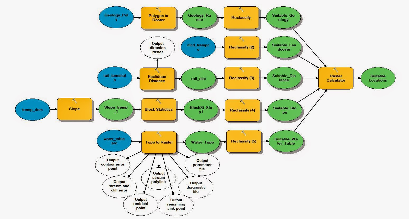Model 1 gives us the suitability of the area based on geology, land cover, distance from a rail terminal, slope, and water table depth.

Model 2

Next we take a look at environmental and community impact criteria. (note all data was provided by the Trempealeau County Database).

Table for model 2 with reclassified categories.

1. Impact on rivers - For the first process I took a shapefile of the Trempealeau River and performed an Euclidean Distance around the feature. I then reclassified the distance with the most impact being closest to the river.

2. Prime Farmland - Next I looked at a feature class of the farmland and created a raster file from the feature class. I then reclassified it to show most impact to prime farmland, medium impact to potentially prime farmland, and least impact to non-prime farmland.

3. Impact on Residential areas - I took a zoning feature class and selected only the residential areas then performed an Euclidean Distance around just those areas. I then reclassified the data with most impact being within 640 meters which is hearing distance and then farther out was least of an impact.

4. Impact on Schools - Next I took a parcel feature class and selected the parcels owned by school districts. I then performed an Euclidean Distance on the data and reclassified them with the most impact being on areas closest to the schools.

5. Factor of choice - Parks - I chose to look at parks for my factor of choice and found a feature class in the Trempealeau geodatabase that worked. I performed an Euclidean Distance on the data and then reclassified the data with the most impact being on areas closest to the park.

6. Viewshed - Horse trails - I chose to use the trails feature class to perform the viewshed and specific chose the horse trails from the trails feature class. I used the DEM from the first section and found most of the area was not seen from these trails. I had most impact as visible and least impact as non-visible.

The model below goes through each of the steps above and then brings them all together with the raster calculator to find the areas that most meet the criteria. This section is opposite to the first section in that the higher the number the most impact the area has from sand mining and the worst that area would be for putting a sand mine in.

Model 2 gives us the environmental and community impact on rivers, prime farmland, residential, schools, and parks that sand mining would have.

Results

So finally I needed to bring both sections together to find the ultimate sand mining locations. I reclassified the first section into three categories 0-5 being the worst, 6-10 being in between, 11-15 being the best. For the second section I needed reclassify the data but first needed to flip the numbers so that the higher numbers were least impact and the lowest numbers were most impact. I then categorized them as 0-5 being the most impact, 6-10 being in between, and 11-15 being the least impact. and with We then used Raster calculator to produce a index number based on all the criteria with the higher the number the more suitable the location would be for sand mining. Lastly, I performed a raster calculator to add the too sections into one raster.

The model below shows the steps to finally bring both sections into one map.

Final model to bring both sections together for the ultimate sand mining locations

The maps below show the results for models 1 and 2 as well as the final model bringing both together into a final map.

Map of the suitability for sand mining based on model 1

Map of the environmental & community impact for sand mining on model 2

Map of both suitability and environmental impact for sand mining on both models

Discussion & Conclusion - The maps above show the areas best suitable and non-impact for sand mining in Southern Trempealeau County. I think that this is a great model for finding a suitable place to build a sand mine (however it is not very realistic). I would find the areas that are recommended in the last map to be good locations they are far from residential areas and won't impact many other factors as well as being suitable for mining sand. I could see some companies using something similar to find a location however, with a lot more detail and more current data.

This overall project this semester has been very interesting and helped me greatly explore skills needed for GIS professionals. I cannot think of a better way to learn and master these skills than the exercises I completed this semester.

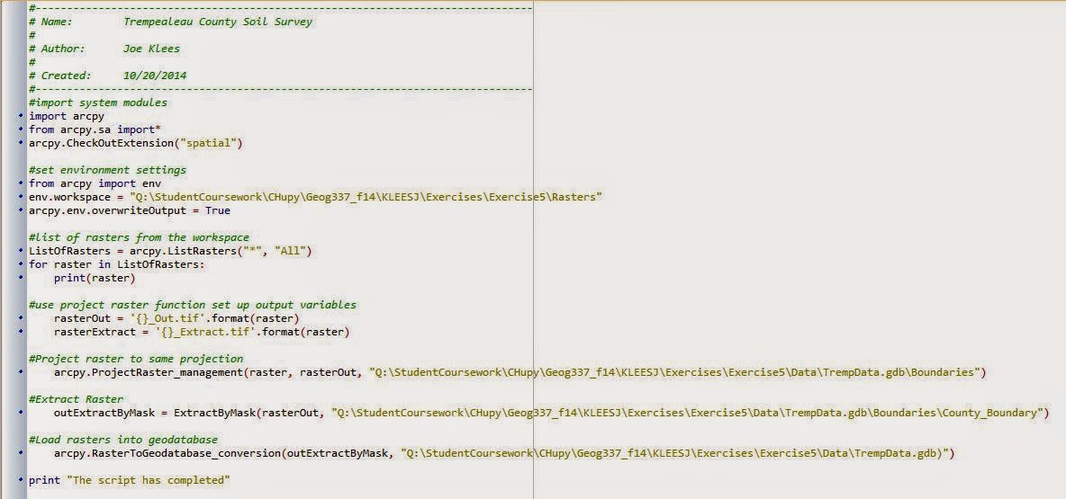
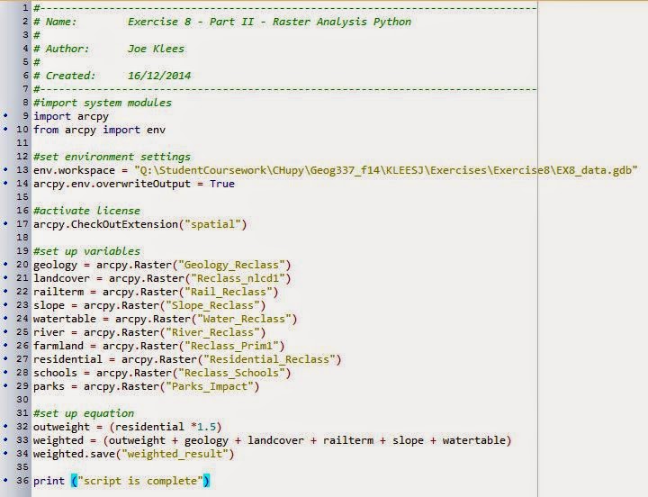
(See Python Blog Post for Python potion of this exercise.)

Exercise 7 - Network Analysis

Introduction - This exercise was focusing on network analysis. We used the example of sand mine locations and finding the fastest route to the closest rail terminal for transportation. We then wanted to estimate the cost that moving all that sand would have on local counties.

Methods - We first wrote a script which can be explained in detail in the python script blog post from October 2014, as well as below. We used this script to select the mines that were farther than 1.5 kilometer from a railroad because those are the mines that we would be trucking their sand to rail terminals.

Python script to select mines farther than 1.5 km away from railroads.

Next we went into ArcGIS and turned on Network Analysis to find the routes between mines and rail terminals. We took a feature class of rail terminals in the country and selected only the ones that used truck and rail. We then took a feature class of street across the country and used Network Analysis to find a route from each mine to the closest terminal. To do this we set the mines as the accidents and rail terminals as the facilities. Once I have the routes as shown in the map in the results section of this blog, I can make a model to find the distance and cost of each route. The model shown below first makes the routes for each mine and then I project the map into 1983 Wisconsin HARN TM (meters) and add the counties feature class. I then use intersect to find the distance of roads traveled by sand-bearing trucks and using summary statistics I find the distance for each county. Next I add and calculate a field to switch the distance from meters to miles. Assuming that each mine makes 50 round trips a year and that each mile costs the county 2.2 cents I add and calculate a field that gives me the cost for each county (100 trips * 2.2 cents * distance traveled in each county). The model is shown below.

Model giving the cost of sand transportation for each county.

Results - The map below shows the locations of the mines in blue circles and rail terminals in green triangles. The routes are the quickest road that trucks can take to go from the mines to the rail terminals.

Map of mine and rail terminal locations with routes

The table below shows each county and the meters and miles traveled by trucks hauling sand and the estimated cost for the county to fix these roads. The cost was found by multiplying the road length in miles by 100 trips and 2.2 cents per mile.

Table of each county with meters and miles traveled by sand trucks and the estimated cost

The table below show the cost for each county with Chippewa County leading by quite a bit.

Discussion & Conclusions - I think that Chippewa County had the most cost due its location in the driftless region that is known for its great sand. Counties that are greatly affected by these trucks and the damage they cause to their roads should think about implementing a tax for these companies to pay in order to use these roads and offset the cost for the counties. However, the cost doesn't seem to high even for counties that are most affected.

Sources
Street data from ESRI streetmap USA
Online Conversion to help with the equation for converting meters to miles.

(See Python Blog Post for Python potion of this exercise.)

Exercise 6 - Data Normalization, Geocoding, & Error Assessment

Introduction - In this exercise we used data from a excel spreadsheet and normalize the data. We then learned how to geocode the data and assess our errors based on our classmates results. The data we were using was addresses of sand mines in Wisconsin for our semester long project on frac sand mining in Wisconsin.

Methods - We first tried to geocode the data using ERSI ArcGIS Online's World Geocode Service. However, since our data wasn't normalized we weren't able geocode any of the addresses. So, we normalized the data by finding the addresses, zip codes, and town for each mine. Many of the sand mines had PLSS addresses so we had to use a school server to find street addresses for those mines that didn't have one. Once we had the data normalized we were able to successfully geocode the address using the World Geocode Service.

Results - Once we geocoded the sand mine locations we were able to map them out in ArcGIS.

The original data before normalization

The data after normalization, ready for geocoding

Map of the geocoded sand mine locations in Wisconsin

Each of us in the class was given about 20 mines to geocode and at the end of the exercise we compared our geocoded mines with those of classmate's who had the same mines. Below is a table of the mines that I geocoded, their name and the distance from my classmate's geocoded location of the same mine.

Mine ID	Facility Name	Distance of my geocoded location from closest classmate's (rounded to the nearest meter)
109	MIDWEST FRAC AND SANDS	0
111	SIOUX CREEK SILICA	0
125	RIVER VALLEY SANDS	14313
136	MUSKIE PROPPANTS	0
138	PREFERRED SANDS	0
151	FG MINERALS (WISCONSIN INDUSTRIAL SAND)	0
152	FG MINERALS LLC	0
163	ATLAS RESIN PROPPANTS, LLC	11383
165	BADGER MINING CORP-TAYLOR PLANT	10603
178	TOWN OF BROCKWAY MINE	0
179	WESTAR PROPPANTS LLC	246
190	BLACK CREEK LIMESTONE CO	3044
192	DIAMOND BLUFF INDUSTRIAL SAND	239
205	ARCARDIA SAND CO	0
206	D95 NORTH SITE - SPARTAN SAND, LLC	1614
218	PATZNER SAND PIT	0
219	PREFERRED SANDS OF WISCONSIN, LLC	2920
232	VERNON BUE SAND MINE	4850
233	FML SAND - READFIELD	3187
245	NORTHERN FRAC SAND LLC	604
246	CHOPPER FARMS	128

Discussion - My data and my classmates' data have low positional accuracy due the uncertainty of certain address were we had rely on PLSS interpretation in order to assign an address to some of the sand mines. There is a inherent error in the data automation and compilation. In some cases there is no knowing which location is correct, however in other cases which show large differences in the data you can see that one or the other point is more accurate based on the PLSS address.

Conclusion - It isn't easy to normalize and geocode addresses especially with a PLSS address instead of a street address.

Exercise 5 - Data Gathering

Introduction - This exercise was focusing on gathering data and we used land cover data for Trempealeau County as an example. There were four steps to this process; downloading the data, importing and joining the data, and then writing a script to project and clip the data.

Data gathering – We downloaded the data from multiple websites:

-          Rail line feature classes from the US Department of Transportation website.

-          An elevation map from the USGS National Map site.

-          An agricultural use map from the USDA Geospatial Data Gateway.

-          Trempealeau County land records from the Trempealeau County Land Records site.

-          Soil information from the USDA NRCS Web Soil Survey.

The websites all gave the data in zipped files and I then extracted them into a common folder. Next I needed to join the attribute tables from the soil survey and the Trempealeau County geodatabase in order to normalize the projection and join the soil information into the land use record. I imported SSURGO data from Microsoft Access in order to join the tables which included a common key for the data to join correctly.

To put the data into a neat map I wrote a Python script which can be seen in the Python scripting blog post under exercise 5. This clipped the data into just the county of Trempealeau and projected the data into the correct projection. It also loaded the finalized feature class into the Trempealeau geodatabase. The resulting map is shown below, incorporating all of the downloaded data into one poster.

Data Accuracy – The table below shows parameters from the metadata for each of the separate data records that were downloaded.

Record	Scale	Effective Resolution	Minimum Mapping Unit	Lineage	Temporal Accuracy
Rail Lines	1:24000	30m	30m	US Department of Transportation	2014
NLCD	1:24000	30m	30m	USGS	2011
DEM	1:100000	10m	10m	USGS	2013
NASS	1:100000	30m	30m	USGS	2013
Trempealeau	1:24000	30m	30m	Trepealeau County Land Records	2014

(See Python Blog Post for Python potion of this exercise.)

Sources:

US Department of Transportation Bureau of Transportation Statisics Link

USGS National Map Viewer Link

USDA Geospatial Data Gateway Link

Trempealeau County Land Records Link

USDA NRCS Web Soil Survey Link

Python Scripting

Introduction - Python is used in writing scripts in ArcGIS to perform data analysis, therefore it is a very important skill to have in the GIS field. This post illustrates some of the skills I learned in writing Python script in my GIS II course.

Exercise 5 - October 20, 2014 - This script was written to project, clip, and load pre-downloaded data into a geodatabase. I input raster data from various website and the output was a clipped map of Trempealeau County in the proper projection and deposited into a pre-designated geodatabase.

Exercise 7 - November 12, 2014 - This script was written to select the active mines, that are not a rail loading station, and not within 1.5 kilometers of the railroads. We used mine and railroad data from DNR, not from our geocoding exercise. Once the script is complete we have a shapefile of the mines that meet the above criteria.

Exercise 8 - December 16, 2014 - This script was written to analyze the raster data that I created in exercise 8 and generate a weighted index model using Python. I first set up the variables, build n equation to weight one of the factors and add all the factors together.

The map below is the resulting raster from the completed python script with the residential being weighted in the overall index with the five suitability factors included.

Exercise 4 - Sand Mining for Hydraulic Fracturing

Introduction

Sand mining is a booming industry in Wisconsin today, and this is because of the increase in Hydraulic Fracturing or fracking that is going on across the country. Wisconsin has some of the best sand in the country and it is vital in the fracking technique. This post is an introduction to the project on sand mining we are doing in this GIS class and will continue throughout the semester.

What is fracking?

Fracking is the mining of natural gas using a hydraulically pressurized liquid full of water, sand, and many other chemicals and fracturing the natural gas contain rocks. This is practiced in areas that have an abundance of shale which is the most common location for natural gas to be stored naturally. The importance of sand mining in Wisconsin is evident in the vital inclusion of sand in the mixture that is used to fracture this shale. Even though the sand mining that is vital to the fracking process is from Wisconsin, fracking does not take place in Wisconsin even though there are some future potential candidates in the northern parts of the state. Rather, the states on the eastern and western coasts as well as southwestern U.S. have the best locations for fracking due to shale formations in these areas.

Where in Wisconsin is the sand mined?

There has been mining of sand in Wisconsin all the way back to the 19th century due the states abundance of the material. Most of the western part of the state is sandstone and the sand here is perfect for fracking because the quartz crystals that make up Wisconsin sand are the correct size and shape needed for fracking. The sandstone reaches from the northern counties of Washburn and Burnett all the way to the southern border of Illinois. The figure below shows the locations of sand mines in Wisconsin mostly focused in the western and central parts of the state. The university here in Eau Claire sits right in the middle of thickest sandstone deposit part of the state.

(fig 1)

Issues with fracking and sand mining

This topic of sand mining and especially fracking are very hot debate issues in the news today. There are issues with what effects there are on the environment when fracking is practiced in the area. Fracking has been related to water contamination, landslides, and other environmental health and safety risks. An article from the Washington Post this past month discussed a recent study that found fracking to increase reports in health problems. The report quotes local farmers near a fracking operation in Arkansas who said they had health problems related to the water they drank believing it to be contaminated by the local fracking. Meanwhile, the companies say that there is no correlation between fracking and public health concern, citing these studies as strictly opinion based polls. However, environmental public health researchers have found there to be some worry but not to make any connections until further research has been done.

How GIS will be used in this project

GIS is an important tool in analyzing spatial data and this can help us get a overview and predict patterns in the data. We can use GIS to map out current sand mines, transportation routes for moving the sand, and future potential mine locations.

Sources 

Robertson JM. 2012. Frac Sand Factsheet. Wisconsin Geological and Natural History Survey.

Paquette D. 2014. Live near fracking? You are more likely to report health problems, new study says. The Washington Post.

Wisconsin DNR. Industrial Sand Mining.

Wisconsin DNR. Silica Sand Mining